Fixing the disconnect in production planning

From the September-October 2025 edition of Supply Chain Management Review.

September-October 2025

This issue of Supply Chain Management Review explores the technologies, strategies, and leadership practices shaping next-generation supply chains. Features include Gartner’s 2025 Top 25 Supply Chains and an…

Browse this issue archive.

Access your online digital edition.

Editor’s Note: Portions of this article are excerpted from Miller and Liberatore (2020) with the permission of Business Expert Press.

Effective and efficient manufacturing operations require close integration between long-run planning and short-run production scheduling. A testament to this is the decades-old field of research and practice titled hierarchical supply chain and production planning (this was called hierarchical production planning in the 1970s), which is devoted to the development of planning frameworks and techniques to integrate long-run planning and short-run scheduling.

To highlight the importance for manufacturing operations of incorporating strong, integrating linkages between medium-term, 12-to-18-month (tactical) planning activities, and shorter-run (operational) production scheduling activities, we offer several examples of production planning/scheduling issues that can arise in the absence of an integrated, hierarchical planning approach. The discussion also illustrates the types of analytical techniques that can link and synchronize long-run plans with short-run schedules.

In this article, we begin with a brief overview of hierarchical production planning. This provides the context and background for the detailed discussion of the short-run/long-run illustrative “linking” methodologies that will follow afterward.

Hierarchical production planning

Hierarchical production planning spans a firm’s entire planning horizon from the strategic, to the tactical, to the operational planning and scheduling levels. Figure 1 presents a hierarchical manufacturing and distribution planning framework (some firms maintain separate planning frameworks for manufacturing and distribution). At this point in the planning process, business strategic plans have been developed and approved, as have the high-level strategic plans of the overall supply chain organization. Now, the manufacturing and distribution functions commence their own strategic planning processes to support the overall supply chain and business unit strategies.    

 

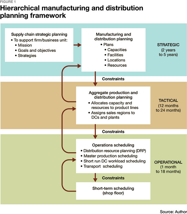
At the strategic planning level, manufacturing must address such issues as planned production capacity levels for the next two years and beyond, the number of facilities it plans to operate, their locations, the resources it will assign to its manufacturing operations, and numerous other important, long-term decisions. Similar decisions must be made for distribution facilities and resources. Decisions made at the strategic level place constraints on the tactical planning level. At the tactical level, typical planning activities include the allocation of capacity and resources to product lines for the next 12 months to 24 months, aggregate planning of workforce levels, the development or fine-tuning of distribution plans, and numerous other activities. Within the constraints of the firm’s manufacturing and distribution infrastructure (an infrastructure determined by previous strategic decisions) managers make tactical planning decisions designed to optimize the use of the existing infrastructure. Planning decisions carried out at the tactical level impose constraints upon operational planning and scheduling decisions. At this level, activities such as distribution resource planning (DRP), rough-cut capacity planning, master production scheduling, shop floor control scheduling, and many other decisions occur.

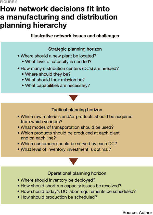
The hierarchical manufacturing and distribution planning (HMD) framework presented in Figure 1 is generic in that although individual HMD systems will differ by firm, most systems are designed within this or a similar general framework. Figure 2 recaps some illustrative generic decisions that an HMD system constructed within this framework will generally address and it displays how these decisions fit into a planning hierarchy. As several of the illustrative decisions in Figure 2 imply, HMD systems typically extend beyond a firm’s internal operations to include decisions about suppliers and customers.         
This completes our brief background review of hierarchical production planning (HPP), and we now turn to several illustrative HPP techniques for linking short-run and longer-run planning, as well as issues that can arise—if planners do not employ appropriate “linking” analytic tools.

 

Product family production planning background

Manufacturing and distribution firms with thousands of unique finished goods end-items typically develop their annual or tactical production and distribution plans at an aggregated product level. Numerous reasons exist for this planning approach, not the least of which is that it is often simply not practical or productive to develop long-run plans (e.g., 12 months to 18 months) for thousands of individual end-items. By aggregating end-items into product families, a planner can avoid creating models so large that they become unmanageable or even mathematically intractable. Figure 3 illustrates the levels of product aggregation which we assume. One can observe that end-items tree up into product families, and product families then tree up into product lines. The examples presented later will assume that the firm’s annual production planning model defines products at the product family level (i.e., level 3 in Figure 3).

 

Product families are created based upon the similarity of one or more key commonly shared characteristics of each end-item within a family. In a production planning industry application for which the author developed a detailed mathematical algorithm incorporating the logic shown in the example that follows, all end-items within each family had virtually identical production rates and production costs. Additionally, to group a set of end-items into one product family, any production line defined for planning purposes as capable of producing a particular product family had to be able to produce each end-item in that product family. This restriction assured that if a long-term production plan (e.g., a 12-month annual plan) assigned a product family to a production line at any plant on the firm’s network, that production line had the capability to manufacture whatever end-items in the product family customers might demand from it. Depending upon the planning application, there exist other characteristics and constraints that one may have to consider when formulating product families for product planning. However, the preceding example depicts the types of considerations that the process of formulating product families must address.

Potential product family: End item disconnect that planning processes must address

Example 1

For illustrative purposes, assume that a firm is developing a 12-month product family production plan for its entire network of manufacturing plants. This plan will specify family production assignments (i.e., production quantities and weeks of production) by plant, by production line, by product family. Inputs that the firm’s planners require include a forecast of demand by product family for the next year, and the current inventory level of each product family.

To determine net production requirements for the next 12 months, planners must subtract the current inventory of each product family from the projected annual demand for that product family. This will yield the actual net production requirements for each product family. The firm bases its annual production plan on these product family net requirements, rather than total demand (i.e., gross requirements). If the firm did not plan production based on net requirements, the inventory of a product family that currently has excessive levels well above target would remain in this costly, overstocked inventory position over the next 12-month planning horizon (safety stock and inventory backorders must also be considered).

To develop the beginning inventory data for each product family in the planning model, planners sum the current inventory of each item in a product family. This aggregation process generates the beginning inventory for each product family in the production planning model.

The following section illustrates the need for a manufacturer to evaluate its inventory at the end-item level across its entire network in order to determine the correct product family beginning inventory level inputs to its annual production planning process. We will observe that determining the net production requirements of end items first (i.e., before developing product family beginning inventories) yields the correct product family beginning inventory planning data. The section includes an example of a mathematical algorithm required to assure synchronization between current manufacturing/distribution network operating conditions and annual/tactical production planning.

Why is it critical to incorporate end-item inventory positions into annual product family level production plans?

It is necessary to evaluate current end-item inventory positions over the entire manufacturing/distribution network in order to assure that the firm’s annual manufacturing plans do not underestimate total production requirements. Inventory data, when developed at the product-family level (rather than at the end-item level), can provide misleading information leading to an underestimation of capacity requirements in long-run planning models.

To illustrate this, assume we are planning the annual production requirements of a product family that has five individual end-items. We now consider the production requirements over a planning horizon for this product family when evaluated at two different levels of inventory aggregation: (1) the end-item level, and (2) the product-family level. To measure the utility of a product family’s current inventory, we require two definitions:

“Usable” inventory over the planning horizon is the minimum of:

1. (forecast annual sales over the planning horizon) + (the end-of-period inventory target), or
2. The current (i.e., beginning-of-period) inventory.

“Excess” inventory over the planning horizon is the maximum of:

1. (current or beginning-of-period inventory) – (usable inventory over the planning horizon), or
2. 0.

A comparison of Figures 4 and 5 reveals that the projected total production requirements over the planning horizon can vary substantially depending on whether one evaluates requirements at the end-item level (column 5, Figure 4: 11,000), or at the product family level (column 4, Figure 5: 8,000). Further, the firm will underestimate its true production capacity requirements if it evaluates inventory at the product family level. In this example, the underestimate of capacity needs will occur because end-item 5 has an extreme surplus of inventory. Because item 5’s current inventory exceeds the sum of its annual selling rate plus inventory target by 3,000 units, the firm will still have an inventory excess of 3,000 units in this item at the end of its 12-month planning horizon. To plan production requirements accurately, the firm must recognize that it has 3,000 units of inventory in item 5 (and therefore in item 5’s product family) which it cannot utilize over the planning horizon. For production planning purposes, including these 3,000 units in the product family’s current inventory figure will overstate the true level of inventory “usable over the planning horizon” for this product family. Thus, the number displayed in column (6) of Figure 4 (8,000), rather than the number in column (5) of Figure 5 (11,000), represents the proper quantity to use as this family’s “beginning-of-period inventory” in an annual production planning model. Obviously for other reasons (e.g., financial, special marketing programs, etc.), one must account for this product family’s excess inventory (over the planning horizon) in other planning areas.

 

 

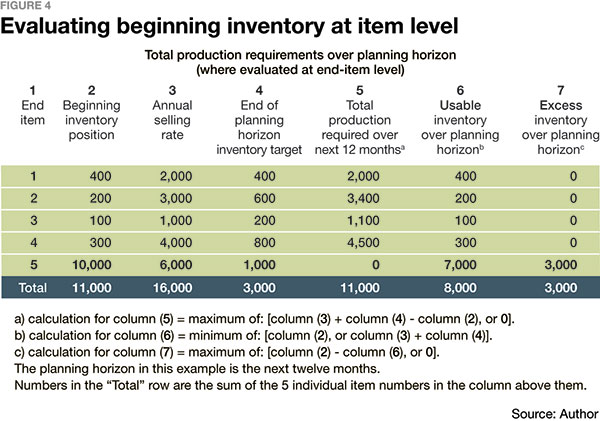
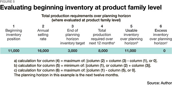
The example in Figure 5 illustrates that evaluating inventory positions (and production requirements) at the product family level makes it impossible to recognize if there is any excess or unusable inventory (over the planning horizon) in any of the end-items within the product family. By using the approach shown in Figure 4, namely, evaluating inventory positions and production requirements at the end-item level, and then summing the end-item results to obtain product family requirements, one can accurately evaluate a product family’s current level of “usable” inventory over the planning horizon.

Algorithm to determine usable and excess inventory over a planning horizon

The example in Figure 4 demonstrates the calculation of usable and excess inventory over the planning horizon for a stand-alone, one location manufacturing/distribution network. In the real world of multi-location networks, the determination of proper usable and excess inventory data for product families becomes more complex. However, the same basic logic used for the one-location network can be extended to a multi-location, multi-echelon network (the author has created an algorithm for just this purpose).

This section has presented a simplistic, yet effective algorithm for developing beginning-of-period inventory data at the product family level for use in production/distribution planning models. The approach described here creates the necessary link to integrate a firm’s short-run, current inventory conditions into its long-run production plans.

Potential product family: End-item disconnect that the planning process must address

Example 2

Our second example of the need for linkages between long-run product family production planning and end-item production scheduling again involves a firm creating a 12-month production plan at the product family level for each plant in its network. Figure 6 displays a network-wide annual production plan that for illustrative purposes we will assume the firm’s planners have created. This plan displays the weeks of production of each product family that each plant will manufacture over a 12-month planning horizon.

 

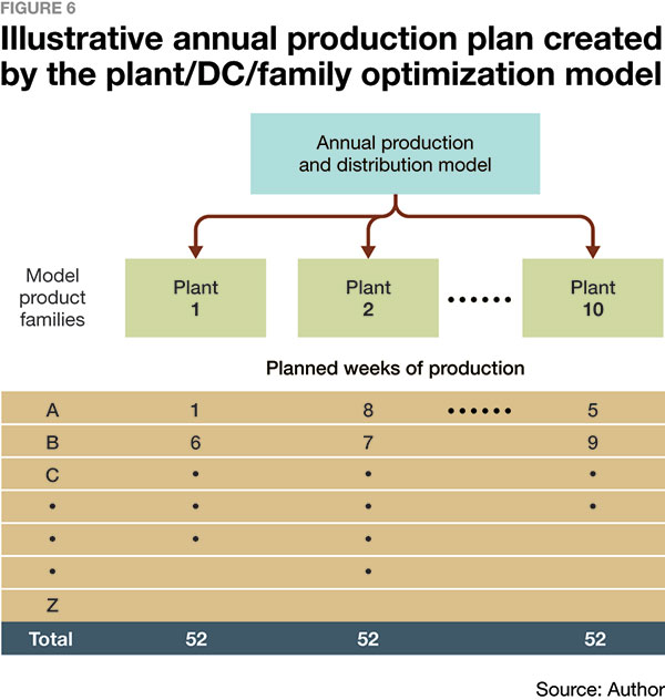
For illustration, we now focus on the plan that Plant 1 should produce one week of product family A. We will also assume that product family A has the following attributes:

1. It contains 20 finished good end-items, and
2. Each of the 20 end-items has a minimum production run length of a 1/2 day (i.e., if the plant has to produce an item, it must produce the item for a minimum of 1/2 of a day).

As previously reviewed, end-items are aggregated into product families for tactical (annual) planning based upon their respective similar characteristics. For example, assume that this is a ceramic tile manufacturing network of plants, and that the 20 end-items in product family A are different color 2-in. x 2-in. wall tile end-items (e.g., blue, green, yellow, etc.). Each end-item can be produced on the same production lines at the same plants, and at very similar costs per unit and at similar output rates. These similar end-items would be planned as one product family in the firm’s production planning model.

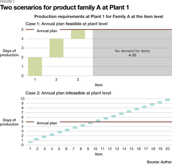
Now let us consider Figure 7, which depicts two very different scenarios (Case 1 and Case 2) under which the firm’s annual production planning model could generate an initial assignment of one week of production for product family A at plant 1. The total demand for product family A consists of the sum of the demand for the 20 end-items that comprise this product family. (For simplicity, we will also define production requirements as equal to total demand in this example.) Now consider Case 1 and Case 2 in Figure 7.

Case 1: The total demand (and production requirements) for product family A at Plant 1 is in three end-items (1, 2, and 3).

• There is no demand for end-items 4 through 20 (i.e., demand = 0)
• Thus, as Figure 7 depicts, to satisfy the demand for product family A at plant 1 will require two days production of item 1, two days of item 2 and one day of item 3.
• Therefore, plant 1 can feasibly produce the production assignment of one week of family A. (Note that we define five business days as one week in this example.)

Case 2: The total demand for product family A at plant 1 consists of 1/4 of a day’s production for each of its 20 end-items.

• 20 x 1/4 = 5 business days total demand; or one week of demand (and production) - the assignment to plant 1 for family A.
• Recall, however, that plant 1 has a minimum production run length of a 1/2 day for any item.
• Therefore, for plant 1 to produce all 20 items in family A it will require 20 x 1/2 = 10 business days (i.e., 2 weeks) of production.
• Thus, the production assignment for plant 1 to produce one week of product family A is not feasible.

 

How infeasible production assignments can occur

At the network-wide tactical (annual) planning level, production models and planners generally do not evaluate very detailed issues such as the minimum run length of individual end-items at individual plants. The purpose and objectives of 12- to 18-month planning exercises at the tactical level necessitate that planning/modeling be conducted at more aggregated levels (e.g., product families rather than end-items).

This allows the possibility that plans developed at the tactical level may, in some cases, be infeasible to implement at the operational level. Case 2 illustrates how these infeasibilities may arise.

In practice, operations personnel from lower planning and scheduling levels must regularly provide feedback to planning personnel at higher tactical levels to avoid the type of situation illustrated in Case 2. As plans cascade down from one planning level to the next lower level (e.g., network-wide to individual plant), managers at the lower level must evaluate these plans and communicate back any infeasibilities.

This becomes an iterative process whereby tactical plans should be revised based on feedback loop communications, and then revised tactical plans are re-evaluated at the operational level. This process continues until a feasible plan, at all levels, is developed.

Finally, note that feedback loops take many forms and can range from: (1) informal communications between two supply chain functions; to (2) formal, standardized data input and output exchanges between functions; to (3) detailed mathematical algorithms that coordinate modeling assumptions and inputs between different planning and operating levels.

Summary

In this article, we first reviewed the concept of hierarchical production planning. HPP is an extremely valuable framework and approach that firms employ to integrate and synchronize their manufacturing activities across their entire planning horizon, from the long-run strategic to the short-run operational.

 We next presented two production examples that illustrate the importance of linking long-run product family-based production planning with short-run end-item scheduling in an integrated, hierarchical approach.

These examples illustrate the types of linkages that firms must develop and ingrain into their manufacturing planning and scheduling processes. Organizations that do not establish these types of links and feedback loops increase their risks of encountering infeasibilities and other execution problems at the operations level. 

About the author

Tan Miller is a supply chain professor in the Norm Brodsky College of Business at Rider University. He previously worked in private industry for more than 25 years where most recently he was responsible for the operations of Johnson & Johnson’s U.S. Consumer Distribution Network. Prior to that, he held a similar role leading the operations of the U.S. Consumer Healthcare Logistics Network of Pfizer Inc. Miller has published eight books and more than 80 articles on supply chain and logistics operations and planning. His most recent books include “Supply Chain Planning: Practical Frameworks for Superior Performance (Second Edition),” and “Logistics Management: An Analytics-Based Approach.”

SC
MR